
Suprafata de raspuns si EVOP
Folosind Minitab®, colaborati cu indrumatorul pentru a crea si analiza experimentul chimic.
Deschideti Minitab®
A. Faza 1:
Selectati: Stat > DOE > Factorial > Create Factorial Design.

Selectati: 2-level factorial (default generators) (2 pana la 15 factori)
Selectati: Number of factors: 2
Selectati: Designs
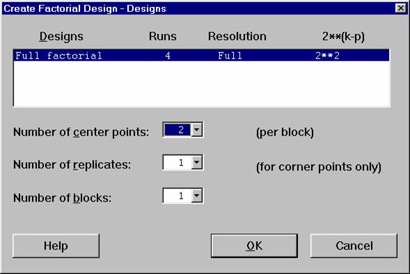
Selectati: Full factorial 4 Full 2**2
Selectati: Number of center points: 2 (per block)
Selectati: OK
Selectati: Factors
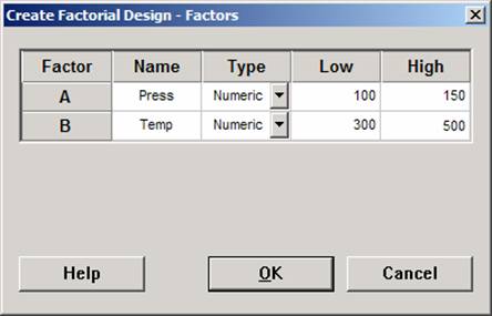
Name Type Low High
Introduceti: Press Numeric 100 150
Introduceti: Temp Numeric 300 500
Selectati: OK
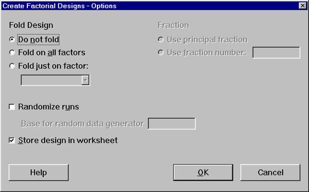
Selectati: Options

Deselectati: Randomize runs
Selectati: OK
Selectati: OK
In fereastra sesiunii vor aparea urmatoarele:
Introduceti datele dupa cum urmeaza:
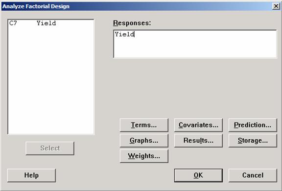
Selectati: Stat > DOE > Factorial > Analyze Factorial Design
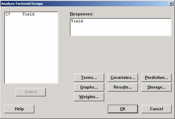
Selectati: Response: Yield
Selectati: Results
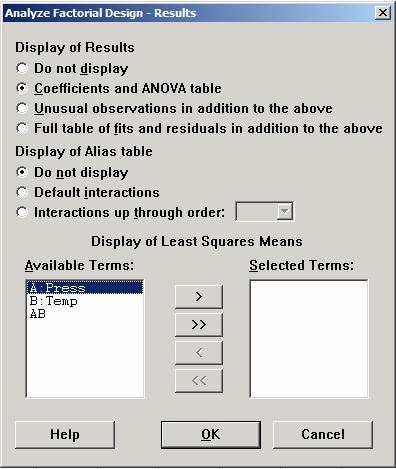
Selectati: Coefficients and ANOVA table
Selectati: Do not display
Selectati: OK
Selectati: OK
In fereastra sesiunii vor aparea urmatoarele:
Factorial Fit: Yield versus Press, Temp
Estimated Effects and Coefficients for Yield (coded units)
Term EffectCoef SE Coef T P
Constant 69.475 0.5303 131.00 0.005
Press17.250 8.625 0.5303 16.26 0.039
Temp-18.450 -9.225 0.5303 -17.39 0.037
Press*Temp -0.750 -0.375 0.5303 -0.71 0.608
Ct Pt 0.575 0.91860.63 0.644
Analysis of Variance for Yield (coded units)
Source DF Seq SS Adj SS Adj MS F P
Main Effects 2 637.965 637.965 318.983 283.54 0.042
2-Way Interactions 10.5630.5630.5630.50 0.608
Curvature 10.4410.4410.4410.39 0.644
Residual Error 11.1251.1251.125
Pure Error 11.1251.1251.125
Total5 640.093
Ce factori sunt semnificativi pentru = 0.10?__________ ______ ____ ______
Curba din testul T este semnificativa pentru = 0.10?_____ _______ ______ _______________
Curba din ANOVA este semnificativa pentru = 0.10?_____ _______ ______ _______________
Suprafata de raspuns este plata sau curba?__________ ______ ____ _______
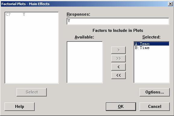
Selectati: Stat > DOE > Factorial > Factorial Plots
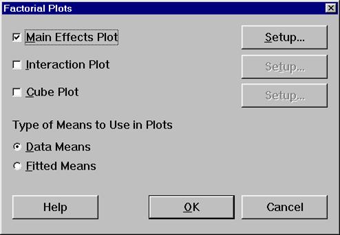
Selectati: Main Effects Plot
Selectati: Setup
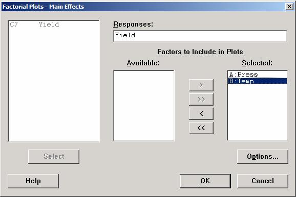
Selectati: Responses: Yield
Selectati: Factors to Include in Plots
Selected:
A:Press
B:Temp
Selectati: OK
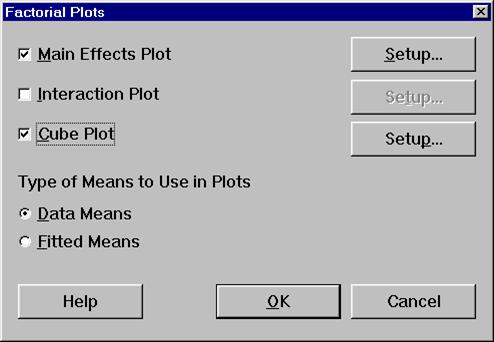
Selectati: Cube Plot
Selectati: Setup
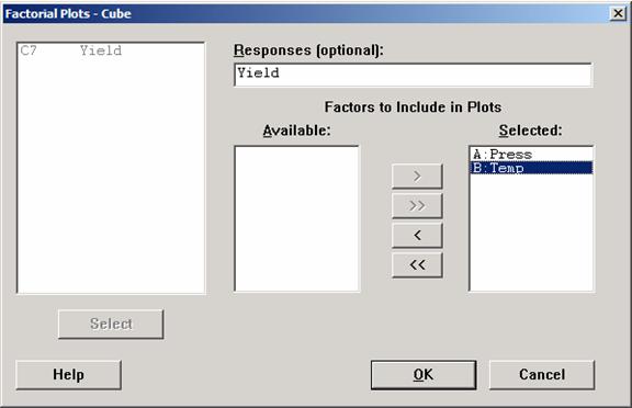
Selectati: Responses (optional): Yield
Selectati: Factors to Include in Plots
Selected:
A:Press
Selectati: OK
Selectati: OK
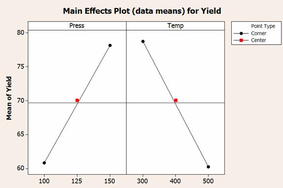
Punctele mediane alcatuiesc o curba? (Da/Nu)
De ce da sau de ce nu?__________ ______ ____ _____ _______ ______ _________
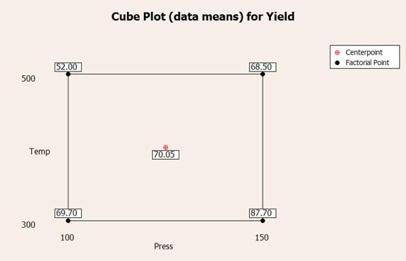
Avand in vedere ca echipa doreste sa maximizeze randamentul, care punct din acest grafic ar trebui sa devina punctul median al noului proiect?_____ _______ ______ __________
Factorii si nivelele pentru faza 2 sunt supa cum urmeaza:
|
Factori |
Nivel -1 |
Pct.median |
Nivel +1 |
|
A: Pres |
125 |
150 |
175 |
|
B: Temp |
200 |
300 |
400 |
Selectati: Stat > DOE > Factorial > Create Factorial Design
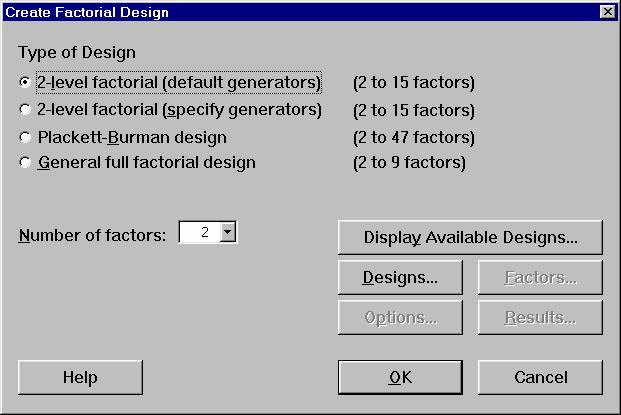
Selectati: 2-level factorial (default generators) (2 to 15 factors)
Selectati: Number of factors: 2
Selectati: Designs
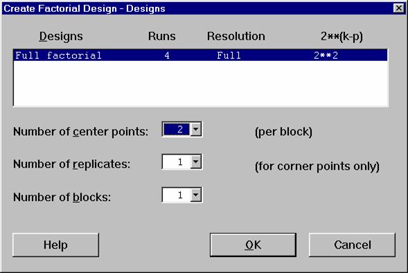
Selectati: Full factorial 4 Full 2**2
Selectati: Number of center points: 2 (per block)
Selectati: OK
Selectati: Factors
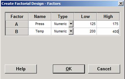
Name Type Low High
Introduceti: Press Numeric 125 175
Introduceti: Temp Numeric 200 400
Selectati: OK
Selectati: Options
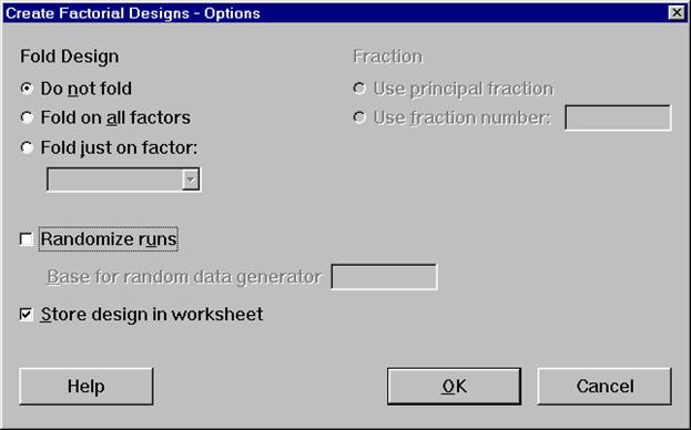
Deselectati: Randomize runs
Selectati: OK
Selectati: OK
In fereastra sesiunii vor aparea urmatoarele:
Introduceti datele dupa cum se arata mai jos:
Selectati: Stat > DOE > Factorial > Analyze Factorial Design
Selectati: Response: Yield
Selectati: Results
Selectati: Coefficients and ANOVA table
Selectati: Do not display
Selectati: OK
Selectati: OK
In fereastra sesiunii vor aparea urmatoarele:
Factorial Fit: Yield versus Press, Temp
Estimated Effects and Coefficients for Yield (coded units)
TermEffectCoef SE Coef T P
Constant78.175 0.3182 245.68 0.003
Press3.650 1.825 0.31825.74 0.110
Temp-3.750 -1.875 0.3182 -5.89 0.107
Press*Temp 7.550 3.775 0.3182 11.86 0.054
Ct Pt9.375 0.5511 17.01 0.037
Analysis of Variance for Yield (coded units)
Source DF Seq SS Adj SS Adj MS F P
Main Effects 2 27.385 27.385 13.692 33.81 0.121
2-Way Interactions 1 57.003 57.003 57.003 140.75 0.054
Curvature 1 117.187 117.187 117.187 289.35 0.037
Residual Error 10.4050.4050.405
Pure Error 10.4050.4050.405
Total5 201.980
Ce factori sau interactiuni sunt semnificativi pentru = 0.10?_____ _______ ______ ________
Curba din testul T este semnificativa pentru = 0.10?_____ _______ ______ _______________
Curba din ANOVA este semnificativa pentru = 0.10?_____ _______ ______ _______________
Suprafata de raspuns este plata sau curba?__________ ______ ____ _______
Selectati: Stat > DOE > Factorial > Factorial Plots
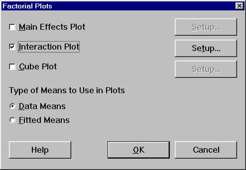
Selectati: Interaction Plot
Selectati: Setup

Selectati: Responses: Yield
Selectati: Factors to Include in Plots
Selected:
A:Press
B:Temp
Selectati: OK
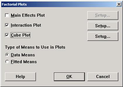
Selectati: Cube Plot
Selectati: Setup
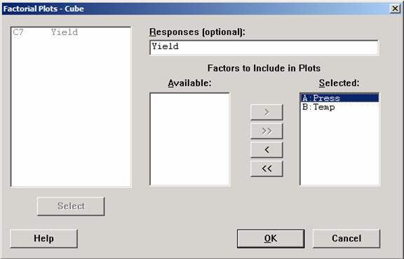
Selectati: Responses (optional): Yield
Selectati: Factors to Include in Plots
Selected:
A:Press
B:Temp
Selectati: OK
Selectati: OK
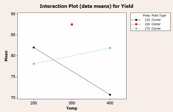
Graficul de interactiune arata o curba? (Da/Nu)__________ ______ ____ ____
De ce da sau de ce nu?__________ ______ ____ _____ _______ ______ _________
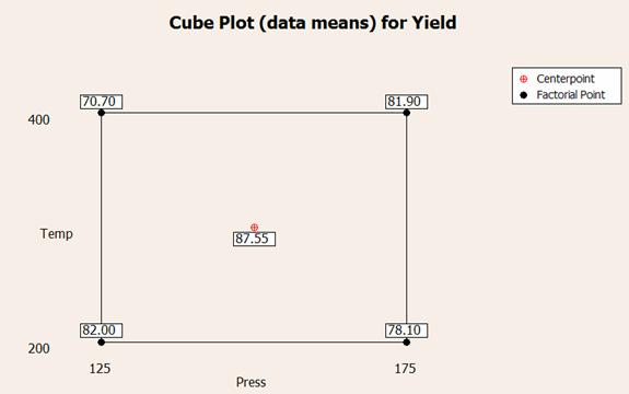
Graficul cubic prezinta o curba? (Da/Nu)__________ ______ ____ __________
De ce da sau de ce nu?__________ ______ ____ _____ _______ ______ _________
Selectati: Stat > DOE > Response Surface > Create Response Surface Design
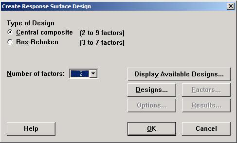
Selectati: Central composite (2 to 9 factors)
Selectati: Number of factors: 2
Selectati: Designs
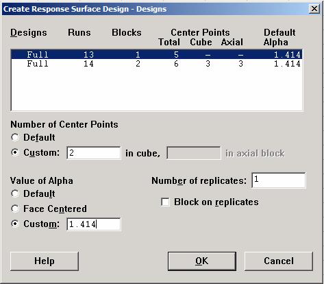
Number of Center Points
Selectati: Custom: 2
Value of Alpha
Selectati: Custom: 1.414
Selectati: OK
Selectati: Factors
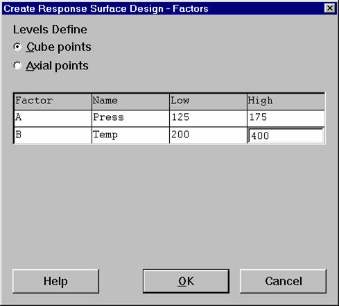
Name Low High
Selectati: Press 125 175
Selectati: Temp 200 400
Selectati: OK
Selectati: Options
Deselectati: Randomize runs
Selectati: OK
Selectati: OK
In foaia de lucru va aparea:
Introduceti datele din experimentul anterior:
Introduceti noile date pentru punctele axiale:
Selectati: Stat > DOE > Response Surface > Analyze Response Surface Design
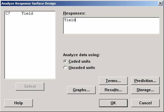
Selectati: Responses: Yield
Selectati: Results
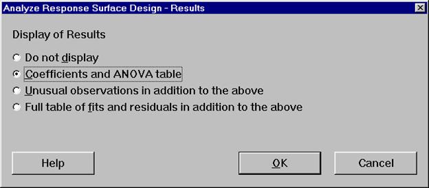
Selectati: Coefficients and ANOVA table
Selectati: OK
Selectati: OK
In fereastra sesiunii vor aparea urmatoarele:
Regresia suprafetei de raspuns: Productivitate versus Pres, Temp
Analiza a fost efectuata folosind unitati codate.
Coeficienti de regresie estimati pentru productivitate
TermCoef SE Coef T P
Constant 87.54912.158 40.576 0.000
Press 2.29151.079 2.124 0.101
Temp -0.38961.079 -0.361 0.736
Press*Press -4.78761.427 -3.354 0.028
Temp*Temp-6.06301.427 -4.247 0.013
Press*Temp3.77501.526 2.474 0.069
S = 3.051 R-Sq = 88.8% R-Sq(adj) = 74.8%
Analiza variatiei productivitatii
Source DF Seq SS Adj SS Adj MS F P
Regression 5 295.038 295.038 59.0076 6.34 0.049
Linear 2 43.216 43.216 21.6078 2.32 0.214
Square 2 194.820 194.820 97.4099 10.46 0.026
Interaction1 57.003 57.003 57.0025 6.12 0.069
Residual Error 4 37.243 37.243 9.3108
Lack-of-Fit3 36.838 36.838 12.2794 30.32 0.133
Pure Error 10.4050.405 0.4050
Total9 332.281
Ce factori sau interactiuni sunt semnificative pentru = 0.10?_____ _______ ______ ________
Modelul a depasit testul LOF?__________ ______ ____ __________________
Sunteti acomodati cu testul LOF?__________ ______ ____ ________________
Curba este in model?__________ ______ ____ _____ _______ ______ __________
De ce da sau de ce nu?__________ ______ ____ _____ _______ ______ _________
Selectati: Stat > DOE > Response Surface > Contour/Surface Plots
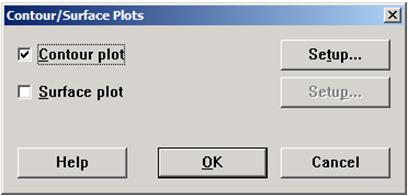
Selectati: Contour Plot
Selectati: Setup
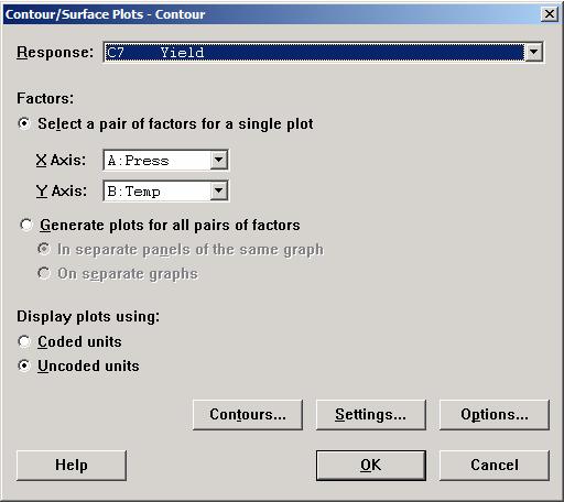
Cele de mai sus trebuie sa fie setate din oficiu.
Selectati: OK
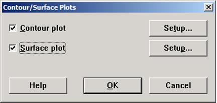
Selectati: Surface plot
Selectati: Setup
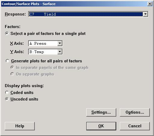
Cele de mai sus ar trebui sa fie setate din oficiu.
Selectati: OK
Selectati: OK
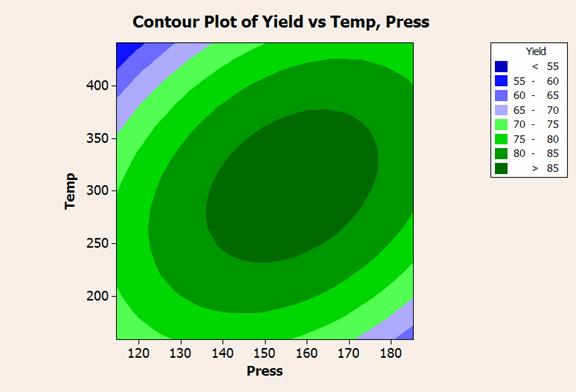
In ce zona poate fi observata productivitatea maxima?_____ _______ ______ ______________
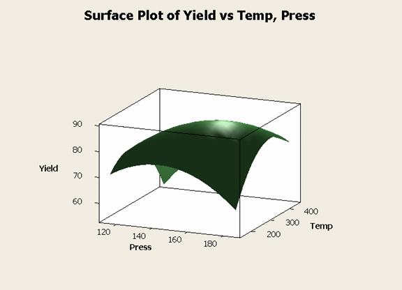
Care ar fi urmatorul (-ii) pas(i)?__________ ______ ____ _________________
1. Grupati-va pe echipe restranse.
2. Completati diagrama. Discutati posibilele schimbari ale setarilor factoriale.
Ciclul 1:
|
Run |
A |
B |
Y |
|
1. |
-1 |
-1 |
28.6 |
|
2. |
+1 |
-1 |
26.0 |
|
3. |
-1 |
+1 |
26.8 |
|
4. |
+1 |
+1 |
25.1 |
|
5. |
0 |
0 |
28.2 |
Schema de codare este:
A: temperatura -1 = 1220 0 = 1240 1 = 1260
![]()

![]()

|
|
Run |
A |
B |
Y |
|
Cycle |
1. |
-1 |
-1 |
28.6 |
|
One |
2. |
+1 |
-1 |
26.0 |
|
|
3. |
-1 |
+1 |
26.8 |
|
|
4. |
+1 |
+1 |
25.1 |
|
|
5. |
0 |
0 |
28.2 |
|
Cycle |
6. |
-1 |
-1 |
29.1 |
|
Two |
7. |
+1 |
-1 |
26.4 |
|
|
8. |
-1 |
+1 |
27.8 |
|
|
9. |
+1 |
+1 |
24.0 |
|
|
10. |
0 |
0 |
27.6 |
Analizati datele folosind Minitab® cu ajutorul urmatoarelor instructiuni. Elaborati un tabel ANOVA, grafice ale tuturor efectelor semnificative si un grafic cubic.
Selectati: Stat > DOE > Factorial > Create Factorial Design
Selectati: 2-level factorial (default generators) (2 to 15 factors)
Selectati: Number of factors: 2
Selectati: Designs
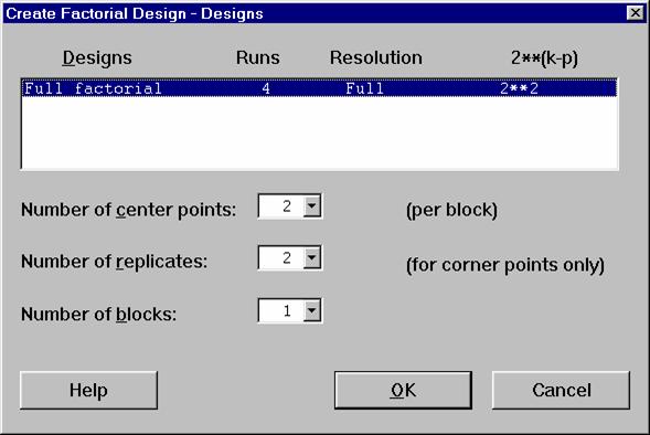
Selectati: Full factorial 4 Full 2**2
Selectati: Number of center points: 2 (per block)
Selectati: Number of replicates: 2 (for corner points only)
Selectati: OK
Selectati: Factors
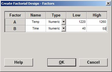
Introduceti: Name Type Low High
Temp Numeric 1220 1260
Time Numeric 40 50
Selectati: OK
Selectati: Options
Deselectati: Randomize runs
Selectati: OK
Selectati: OK
In foaia de lucru ar trebui sa apara urmatoarele:
Selectati: Stat > DOE > Display Design
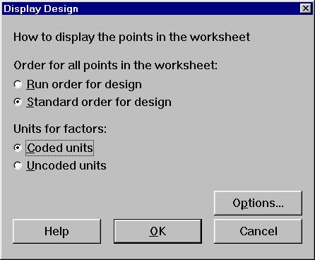
Selectati: Order for all points in the worksheet:
Standard order for design
Selectati: Units for factors:
Coded units
Selectati: OK
Foaia dvs. de lucru ar trebui sa arate astfel:
Adaugati datele in foaia dvs. de lucru in spatiile adecvate:
Selectati: Stat > DOE > Factorial > Analyze Factorial Design
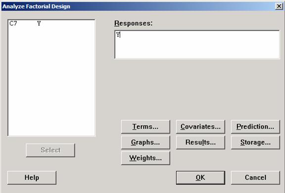
Selectati: Responses:
Y
Selectati: Terms
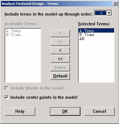
Selectati: Selected Terms:
A:Temp
B:Time
AB
Selectati: Include center points in the model
Selectati: OK
Selectati: Results
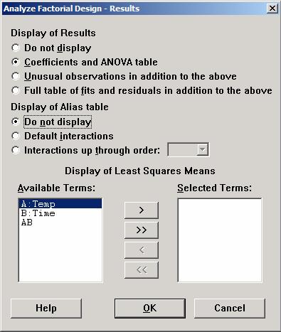
Selectati: Display of Results
Coefficients and ANOVA table
Selectati: Display of Alias table
Do not display
Selectati: OK
Selectati: OK
In fereastra sesiunii ar trebui sa apara urmatoarele:
Factorial Fit: Y versus Temp, Time
Estimated Effects and Coefficients for Y (coded units)
Term EffectCoef SE Coef T P
Constant 26.725 0.1930 138.47 0.000
Temp -2.700 -1.350 0.1930 -6.99 0.001
Time -1.600 -0.800 0.1930 -4.15 0.009
Temp*Time -0.050 -0.025 0.1930 -0.13 0.902
Ct Pt 1.175 0.43162.72 0.042
Care factori sunt semnificativi?
1. Interactiunea este semnificativa?
2. Curba este prezenta (center pt. significant)?
Creati garficul efectelor principale si graficul cubic:
Selectati: Stat > DOE > Factorial > Factorial Plots

Selectati: Main Effects Plot
Selectati: Setup
Selectati: Responses:
Y
Selectati: Factors to Include in Plots:
Selected:
A:Temp
B:Time
Selectati: OK
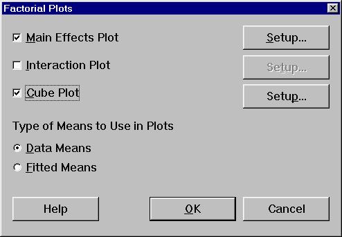
Selectati: Cube Plot
Selectati: Setup
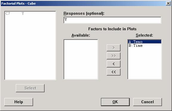
Selectati: Responses:
Y
Selectati: Factors to Include in Plots:
Selected:
A:Temp
B:Time
Selectati: OK
Selectati: OK
Ar trebui sa apara urmatoarele grafice ale efectelor principale:
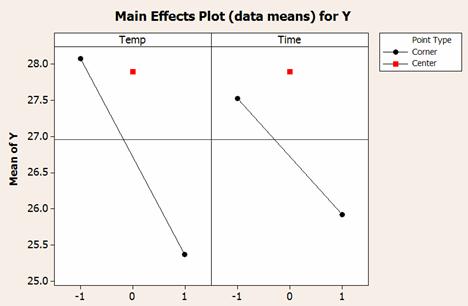
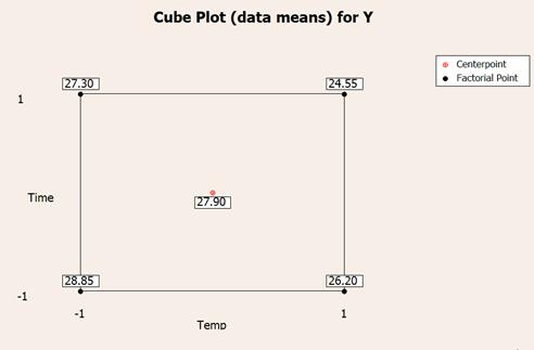
Trebuie sa apara urmatorul grafic cubic:
Elaborati, sub forma de diagrama, punctele pentru Faza 2 (incercarea de a maximiza Y) si noua schema de codare.
![]()

|
Politica de confidentialitate |
| Copyright ©
2024 - Toate drepturile rezervate. Toate documentele au caracter informativ cu scop educational. |
Personaje din literatura |
| Baltagul caracterizarea personajelor |
| Caracterizare Alexandru Lapusneanul |
| Caracterizarea lui Gavilescu |
| Caracterizarea personajelor negative din basmul |
Tehnica si mecanica |
| Cuplaje - definitii. notatii. exemple. repere istorice. |
| Actionare macara |
| Reprezentarea si cotarea filetelor |
Geografie |
| Turismul pe terra |
| Vulcanii Și mediul |
| Padurile pe terra si industrializarea lemnului |
| Termeni si conditii |
| Contact |
| Creeaza si tu |