OPTIMIZATION OF A PHOTOCATALYTIC DECOLORIZATION PROCESS BY USING GENETIC ALGORITHMS

Abstract

This paper proposes a genetic algorithm and neural network based procedure for estimation the optimal conditions for a dyestaff wastewater treatment process consisting of a heterogeneous photocatalytic oxidation.

A simulated dyestaff effluent containing the azo dye Reactive Black 5 (RB5) is decolorized by a photocatalytic reaction using TiO₂ P-25 as catalyst in the presence of Fe⁺³ and H₂O₂. The 16 series of experimental data obtained in different conditions constitute the training and validation data sets for neural network modeling. A simple feed forward neural network with two hidden layers was projected and used to predict evolution in time of the decolorization of this type of wastewater.

In the second stage, the neural model was included in the optimization procedure solved with a simple genetic algorithm. The goal of the optimizations is to calculate the optimal reaction conditions (illumination time and amounts of reagents) which assure an imposed value for the transmittance.

Keywords: neural network modeling, genetic algorithm optimization, wastewater, photocatalysis, RB5, dye.

Introduction

The elimination of toxic chemicals from wastewater is presently one of the most important subjects in pollution control. These pollutants may originate from industrial applications (petroleum refining, textile processing etc.) or from household and personal care areas (pesticides and fertilizers, detergents etc.); several of them are resistant to conventional chemical and biological treatment methods. The search for effective means of removing these compounds is of interest to regulating authorities everywhere.

The textile dyeing and finishing industry is one of the major pollutants among the industrial sector, since modern dyes are characterized by great stability and a large degree of aromatics in their structure. Almost 30 % of the amount of dyes used is released in the wastewater, so these are highly coloured and with a great organic matter (Easton, 1995; Forgacs et al., 2004). The nonbiodegradability of textile wastewater is due to their high content of dyestuffs, surfactants and other additives. Due to the stability of modern dyes, conventional biological treatment methods for industrial wastewater are ineffective, frequently resulting in an intense coloured discharge from the treatment facilities. Additionally, they are readily reduced under anaerobic conditions to potentially hazardous aromatics. Thus, there is a need for developing more effective treatment methods in eliminating dyes from a waste stream at its source.

Heterogeneous and homogeneous solar photocatalytic detoxification methods (TiO₂/H₂O₂, Fe⁺³/H₂O₂) have shown recently great promise for the treatment of industrial wastewater, groundwater and contaminated air. Additionally, the semiconductor mediated photocatalytic process has shown also great potential for disinfection of air and water, thus making possible a number of applications (Peral et al., 1997; Alfano et al., 2000; Malato et al., 2003).

General description of heterogeneous and homogeneous photocatalysis under artificial or solar irradiation is presented in several excellent review articles (Serpone et al., 2002; Hoffman et al., 1995; Fujishima et al., 2000; Herrmann et al., 1999). A brief summary is presented here only for the sake of completeness.

It is well established that by the irradiation of an aqueous TiO₂ suspension with light energy greater than the band gap energy of the semiconductor (Eg > 3.2 eV), conduction band electrons (e^-) and valence band holes (h⁺) are generated. Part of the photogenerated carriers recombine in the bulk of the semiconductor, while the rest reach the surface, where the holes, as well as the electrons, act as powerful oxidants and reductants, respectively. The photogenerated electrons react with the adsorbed molecular O₂ on the Ti(III)-sites, reducing it to superoxide radical anion O₂^.-, while the photogenerated holes can oxidize either the organic molecules directly, or the OH^- ions and the H₂O molecules adsorbed at the TiO₂ surface to OH^. radicals. These radicals together with other highly oxidant species (e.g. peroxide radicals) are reported to be responsible for the primary oxidizing step in photocatalysis. The OH^. radicals formed on the illuminated semiconductor surface are very strong oxidizing agents, with a standard reduction potential of 2.8 V vs NHE. These can easily attack the adsorbed organic molecules or those located close to the surface of the catalyst, thus leading finally to their complete mineralisation. The efficiency of the heterogeneous photocatalytic degradation   onto TiO₂, is strongly dependent on the experimental conditions, e.g., presence or absence of oxygen, temperature, catalyst and substrate concentrations, pH, light intensity, presence of electron donors and acceptors. Also the dissolved metal ions such as Fe⁺³- ions present in the natural and waste waters can significantly modify the purification process.

Although it is well known for some time that the Fenton reagent, a mixture of Fe⁺² salts and H₂O₂, can easily oxidize organic compounds, it has been applied for water and soil treatment only during the last years (Chamarro et al., 2001; Bidga, 1995; Lee et al., 2001). This reagent is an attractive oxidative system, which produces in a very simple way OH^. radicals (eq. (1)) for wastewater treatment, due to the fact that iron is a very abundant and non toxic element and hydrogen peroxide is easy to handle and environmentally safe. Furthermore it was found that the reaction can be enhanced by UV/VIS light (artificial or natural), producing additional OH^. radicals and leading to the regeneration of the catalyst (eq. (2)) (Photo-Fenton reaction) (Oliveros et al., 1997; Fallmann et al., 1999; Arana et al., 2001).

Fe⁺² + H₂O₂Fe⁺³ + OH^- + OH^. 

Fe⁺³ + H₂O + hv (<450 nm) Fe⁺² + H⁺ + OH^. 

These reactions are known to be the primary forces of the photochemical self-cleaning of atmospheric and aquatic environment (Faust et al., 1993).

The photocatalytic degradation of azo dyes containing different functionalities has been reviewed using TiO₂ or the Photo-Fenton reagent as photocatalysts in aqueous solutions under solar and UV-A irradiation (Muruganandham et al., 2006; Augugliaro et al., 2002; Neppolian et al., 2002). The combination of both processes, as has been reported by other authors (Marugan et al., 2006; Mrowetz et al., 2004), leads to an enhancement of the removal rate of the pollutants due to the fact that Fe⁺³ ions and H₂O₂ act as scanvengers of the electrons, which are photogenerated in the conduction band of TiO₂, while the produced Fe⁺² ions can participate again in the Fenton reaction (eq. 1).

The phenomenological treatment of such photochemical systems are very complex. In general, the rate of reaction in heterogeneous photocatalytic systems is a complex nonlinear function of catalyst loading, light intensity, initial solution pH, reactant and oxidants concentration,   etc. Due to these reasons, the ability of systems such as neural networks (NN) to recognize and reproduce cause-effect relationships through training, for multiple input-output systems, has gained recently popularity, in various areas of chemical engineering (Ozkaya et al., 2007; Torrecilla et al., 2007), also in the field of photocatalytic treatment of wastewater (Pareek et al., 2002; Duran et al., 2006; Toma et al., 2004; Salari et al., 2005).

The solution of an optimisation problem can be found through, among others, deterministic or stochastic approaches. The former composes the traditional optimisation methods (direct and gradient-based methods) and have the disadvantages of requiring the first and/or second-order derivatives of the objective function and/or constraints or of being not efficient in non-differentiable or discontinuous problems. Furthermore, the deterministic methods are dependent on the chosen initial solution and can tend to converge towards local extrema of the fitness function, which is clearly unsatisfactory for problems where the fitness varies non-monotonously with the parameters. The stochastic methods, such as genetic algorithms (GA), do not possess these drawbacks. GAs are part of the so-called evolutionary algorithms and compose a search and optimisation tool with increasing application in scientific problems. They do not need to have any information about the search space, just needing an objective/fitness function that assigns a value to any solution (Deb, 1999).

In recent years, due to the rapid progress in computing technology available, there is a growing interest in optimization techniques based on genetic and evolutionary algorithms. The basic algorithm, simple GA or SGA, offers advantages over more traditional optimization approaches (e.g. several search techniques, Pontryagin's principle, SQP etc.), in some cases. Moreover, it has the advantages that it does not require good initial guesses for the values of the decision variables. It uses a population of several points simultaneously along with probabilistic operators (reproduction, crossover and mutation), inspired by natural genetics. Additionally, SGA has the advantage that it uses only the values of the objective functions and not any derivatives, as required by gradient search techniques (Guria et al., 2005).

Because of their flexibility, ease of operation, minimal requirements and global perspective, these algorithms have been successfully used in a wide variety of problems (Deb, 2001) GA has found various applications in chemical engineering including process control, gas pipeline design, pattern recognition of multivariate chemical data, optimization of reaction rate parameters, multipurpose chemical batch plant design, and scheduling (Yan et al., 2003) Details about different types of genetic algorithms - simple genetic algorithm or different adaptations for problems with multiple constraints - and a series of their applications in optimization of the chemical processes has been descried in the reviews of Bhaskar (2000) and Nandasana (2003).

The main goal of this paper is to develop a general procedure based on neural networks and genetic algorithms which could be applied to the complex optimization problems. Neural networks are used as efficient modeling tool and genetic algorithms as solving method of optimization; a neural model of the process is included in the optimization procedure. The case study is the estimation of the evolution in time of a dyestuff wastewater treatment process consisting of a photocatalytic oxidative reaction. It is followed a certain decolorization degree related to optimal working conditions: illumination time, amounts of catalyst TiO₂ P-25, H₂O₂ and Fe⁺³. The GA optimization procedure has proved easily to apply with useful and accurate results.

Experimental

Reagents

This synthetic wastewater (CSW) was made according to recipe used for dyeing of cotton fabrics and was of the following composition 0.07 g L^-1 Reactive Black 5, 0.1 g L^-1 HCOOH, 0.250 g L^-1 Perydrol FHB 15 %, 0.375 g L^-1 Sequion, 0.5 g L^-1 Na₂CO₃, 0.5 g L^-1 NaOH, 3 g L^-1 NaCl. The CSW has an initial pH value of 12 and a DOC of 0.15 g L^-1 (0.5 g L^-1 COD and 0.12 g L^-1 BOD₅).

TiO₂ P-25 of Degussa (anatase/rutile = 3.6/1, surface area 56 m² g^-1 nonporous) was used for all photocatalytic experiments. All other reagent-grade chemicals, such as FeCl₃ ^. 6 H₂O, H₂O₂ etc., were purchased through Merck and were used without further purification.

Procedures and analysis

Experiments were carried-out in a closed Pyrex cell of 500 ml capacity, provided with ports, at the top, for bubbling air necessary for the reaction to take place. The reaction mixture was maintained as suspension by magnetic stirring. Previously to irradiation, the reaction mixture was left 15 minutes in the dark with the aim at achieving the maximum adsorption of the dye onto the semiconductor catalyst surface. The irradiation was performed with a 9 W central lamp. The spectral response of the irradiation source (Osram Dulux S 9W/78 UV-A) according to the producer is ranged between 340 and 400 nm with a maximum at 366 nm and two additional weak lines in the visible region. The photon flow per unit volume of the incident light was determined by chemical actinometry using potassium ferrioxalate. The initial light flux, under exactly the same conditions as in the photocatalytic experiments, was evaluated to be 1.16 x 10^-4 Einstein min^-1.

In all cases, during the experiments, 500 ml of a acidified (pH_o=3.2) dye solution containing the appropriate amounts of semiconducting powder, H₂O₂ and Fe⁺³ was magnetically stirred before and during irradiation. Specific quantities of samples were withdrawn at periodic intervals and filtered through a 0.45 mm filter (Schleicher and Schuell) in order to remove the catalyst particles. With the aim at assessing the extent of color removal, changes in the concentration of Reactive Black 5 were observed from its characteristic absorption band at 585 nm, using a UV-VIS spectrophotometer Shimadzu UV-160 A. The pH values of the solution were monitored with a Metrohm pH-meter, while the reaction temperature was kept constant at 25 0.1 ⁰C.

Formulation of the optimization problem

In complex chemical processes, the ability to select optimum operating conditions in the presence of multiple conflicting objectives, given the various constraints of the process, can present a major challenge. The general solution of an optimization problem can be obtained in terms of the following four elements: an accurate model of the process, a selected number of control variables, an objective function and a suitable numerical method for solving the specified optimization problem.

A good process model is a prerequisite for application in the optimal control strategy. The modeling with neural networks has a series of advantages: the possibility to apply this method to complex non-linear processes, the ease in obtaining and using these models, the possibility to substitute experiments with predictions. Neural networks possess the ability to learn what happens in the process without actually modeling the physical and chemical laws that govern the system. Neural models need only input-output data (experimental or simulation data) so, their advantages are evident against the complexity of the computation.

GAs have several characteristics that make them attractive to solve optimization problems where the model is only available in an implicit form (black-box model). Firstly, due to the fact they are based on a direct search method, it is not necessary to have explicit information of the mathematical model or its derivatives. Secondly, the search for the optimal solution is not limited to one point but it rather relies on several points simultaneously, therefore the knowledge of initial feasible points is not required and such points do not influence the final solution (Leboreiro et al., 2004).

A series of experiments have been carried out for the decolorization of the synthetic dyestaff effluent containing the Reactive Black 5 (RB5) as a model azo dye, by photocatalytic degradation using TiO₂ P-25 as catalyst in the presence of Fe⁺³ and H₂O₂. Based on these experimental data, a neural modeling methodology was developed to describe the dependence of the water decolorization process of different reaction conditions and irradiation time. A MLP(4:9:3:1) - feed-forward neural network with 4 variables as inputs (illumination time in min, amount of catalyst TiO₂ P-25, g L^-1, amount of H₂O₂ and Fe⁺³ mg L^-1), two intermediate layers with 9 and 3 neurons, respectively, and one output - transmittance in %, is designed for process modeling (figure 1).

Figure 1

The feed-forward, multilayered neural network is the most used network's type because the simplicity of its theory, ease of programming, good results and for its universal function in the sense that if topology of the network is allowed to vary freely it can take the shape of any broken curve.

The model MLP (4:9:3:1) was tested against training and validation data. Good agreement between experimental data and neural network predictions (average relative errors less than 1.5 % and correlation over 0.99) proves that the neural model is convenient for the optimization procedure. Details concerning the development and testing this model were given in a previous paper (Suditu et al., 2007).

In this study, the optimization problem includes the neural model which is represented as:

NN [Inputs: t, TiO₂, H₂O₂, Fe⁺³ ; Output: D] (3)

The vector of control variables , u, has the components:

u = [t, TiO₂, H₂O₂, Fe⁺³] (4)

An admissible control input u* should be formed in such a way that the performance index, J, defined by the following equation, are minimized:

(5)

subject to:

(6)

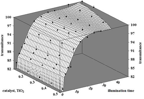
with t representing illumination time, D_f - transmittance at the end of the process and D_d - an imposed value for this parameter.

The transmittance is a measure of the dye elimination from wastewater, with values between 0 and 100 %. High values for this parameter mean high degree of dye elimination.

The constraints are very important to define the range of variation of parameters and to disregard possible solutions that could be interesting in a theoretical approach to the problem.

In other words, the optimization problem to be solved can be formulated as: Which are the optimal working conditions (time, amount of catalyst TiO₂ P-25, amounts of H₂O₂ and Fe⁺³) necessary to obtain an imposed transmittance under the given experimental conditions?

The optimization procedure includes a neural model and it is solved with a simple genetic algorithm. The fitness function of the GA is the scalar objective function (5). Figure 2 illustrates this optimization procedure. Genetic algorithm provides, after an iterative calculus, the optimal values for decision variables (time, TiO₂, H₂O₂, Fe⁺³), which are the inputs for the neural network model. With these inputs, the neural network computes the final value of transmittance, D_f which will be compared with the desired value, D_d. If the two values are identical or there is a very tight difference between them, we can conclude that the task of the optimization, represented by minimum of the objective function, J, is achieved.

Figure 2

GA optimization technique

Genetic algorithms are intelligent stochastic optimization techniques based on the mechanism of natural selection and genetics. GAs start with an initial set of solutions, called population. Each solution in the population is called a chromosome (or individual), which represents a point in the search space. The chromosomes are evolved through successive iterations, called generations, by genetic operators (selection, crossover and mutation) that mimic the principle of natural evolution. A set of solutions are analyzed and modified by genetic operations simultaneously, where selection operator can select some "good" solutions as seeds, crossover operator can generate new solutions hopefully retaining good features from parents, and mutation operator can enhance diversity and provide a chance to escape from local optima (Wang et al., 2006). In a GA, a fitness value is assigned to each individual according to a problem-specific objective function. Generation by generation, the new individuals, called offspring, are created and survive with chromosome in the current population, called parents, to form a new population.

In our GA model, we used real values encoding for the chromosomes. There are other approaches for genetic algorithm based optimization which use binary solution representation, as it is the simplest type of encoding, in which chromosomes are composed only of 1's and 0's. Even the number of alleles is thus rather small (two), this encoding is very common, because it is very easy to use. However, value encoding is more general, because genes are real numbers. Some experiments (Michalewicz, 1996) have shown that real value encoding is more time efficient, with better precision of the solutions.

The initial population is generated randomly. Offspring are created by genetic operators and it is stored in a population pool that is a collection of offspring and their parents.

Selection compares the chromosomes in the population aiming to choose those which will take part in the reproduction process. The selection occurs with a given probability on the base of fitness functions. The fitness function plays a role of the environment to distinguish between good and bad solutions. The individuals with higher fitness must have more chances to reproduce. For each individual to be created in the next generation, two parents are thus selected.

There are different methods for selection phase; our paper uses rank selection which first ranks the population and then every chromosome receives fitness from this ranking. The worst will have fitness 1, second worst 2 etc. and the best will have fitness n (number of chromosomes in population).

The probability that the individual i should be chosen in the rank selection is:

(7)

where rank(i) is the rank assigned to each individual i, determined as an index in the population ordered on the basis of the fitness; n is the number of individuals within the population (in the case considered here, n = 50); a_rank b_rank and b_rank is a parameter that could be controlled by the user, with b_rank (b_rank = 2 in this work).

The recombination (crossover) has as main purpose the recombination the features of two randomly selected parents from the mating pool with the aim of producing better offspring.

Arithmetic real value crossover produces a linear combination of the parents. Given a uniform random number ,

(8)

or

(9)

where C is the real value chromosome of the child, and M and F are the chromosomes of the parents.

The variant of crossover used in this study supposes different points for all genes, that means the new individual will no longer be on the line segment that links its parents. The r value is different for every gene. The offspring will look more like one parent regarding a feature and less regarding another.

After recombination, offspring undergoes to mutation. Generally, the mutation refers to the creation of a new chromosome from one and only one individual with predefined probability. Mutation is used to produce small perturbations on chromosomes to promote diversity of the population.

Our GA includes a variant of mutation named resetting. A gene value is reset to a random value in its search interval. The purpose is to refresh the search process, in case when the genetic diversity of the population decreases (so no longer converges to the solution) or the algorithm has converged into a local optimum. Each gene is independently considered, and mutation gives it a new random value in the initialization interval. Only some genes change (possibly all, but unlikely).

After the three operators are carried, the offspring is inserted into the population, replacing the parent chromosomes in which they were derived from, producing a new generation. The best individual is copied directly into the new population (the elitism technique) and the rest of the individuals are replaced by the new generations. So, in order to keep the best solution, we have considered an elitism factor f_e = 1, that is the best individual is copied directly in the new generation. That ensures that the overall solution of the GA will not get worse.

The termination criterion determines when GA will stop. In other words, the genetic operations are repeated until a termination condition is met. In our implementation, we stopped GA if the maximum number of generations has been executed or the pre-set number of generations without improvement in the last best solution has been reached.

Results and discussions

Population size, number of generations, crossover probability and mutation probability are known as the control parameters of genetic algorithms. The values of these parameters must be specified before the execution of GA and they depend on the nature of the objective function. One important thing in using GA as solving method is to adjust its parameters to the particular problem approached so as to obtain good solutions and to preserve the algorithm from a preliminary convergence.

There is no general termination criteria for GA. Predetermined number of generations, time or comparison of the best solutions to average fitness may be taken as stopping criterion. In our work, the number of generations is established before running and constitutes the stop criterion.

Several tests lead to the following values: pop_size = 50 (size of initial population), max_gen = 100 (maximum number of generations), cross_rate = 0.9 (rate of crossover) and mut_rate = 0.03 (rate of mutation).

The fitness function in GA is the objective function of the optimization procedure. The results of the optimization are represented by the values of the decision variables (illumination time, amounts of catalyst, H₂O₂ and Fe⁺³) that lead to a minimum value of the objective function, which means the achievement of the imposed value for the transmittance.

The optimization procedure is implemented in Matlab 7.0 with original software, as specific functions were programmed for each phase of the genetic algorithm.

Since GA is a stochastic algorithm, we run it for many times, for each situation (each row in the tables of results) to get statistically meaningful values for the time taken. Longer runs are not necessary as GA is already a population based procedure that works with multiple solutions. One of the solutions (the best solution) is chosen and inserted into the results tables.

The variation domains for decision variables are represented by the constraints (6). Imposing different values for transmittance, in the interval 75 % 100 %, the optimal working conditions obtained by GA optimization procedure are given in Table 1.

Table I

In all cases in Table I, D_f = D_d, that means the goal of the optimization has been accomplished.

Taking into account that TiO₂ P-25 is the   expensive component, the same simulations are repeated for a smaller interval, 0.1 - 0.3 g L^-1 TiO₂. Good results are obtained in this situation too, with D_f = D_d (Table II).

Table II

Therefore, the results in Tables I and II represents the optimal working conditions (illumination time, amounts of catalyst, H₂O₂ and Fe⁺³) necessary for obtaining a pre-established value for transmittance. It was expected that high values for transmittance involve higher amounts of reagents and longer illumination time.

Supplementary calculations were added to data in Tables I and II concerning the energy necessary for the decolorization process composed from the energy consumed by the light source and for the mixture stirring. Tables III and IV are the correspondents for Tables I and II, respectively, and the results are in decreased order by the energy. In each table, two values were marked with grey bands, they having small necessary energy and relatively high values for transmittance (small ratio c/c₀, respectively, where c is the concentration of the dye and c₀ - initial concentration). In Table III, the domain for the amount of catalyst was 0.1 - 1 g L^-1 and in Table IV this domain was narrower, 0.1 - 0.3 g L^-1.

Table III

Table IV

Other types of optimizations performed in this paper uses the same objective function with an imposed value for transmittance and, in addition, a supplementary constraint - a pre-established value for amount of catalyst, TiO₂ P-25. In these conditions, GA method determines optimal values for the following three decision variables: illumination time, amount of H₂O₂ and amount of Fe⁺³. The neural model included into the optimization computes the final value for transmittance, D_f, in order to compare it with the desired value, D_d. The variation domain of the parameters were: time = 0 60 min, H₂O₂ = 100 800 mg L^-1, Fe⁺³ = 1 65 mg L^-1, D_d = 80 100 %, step 1 and TiO₂ P-25 = 0.1 1 g L^-1, step 0.1. Several examples are presented in Table V. Even the restrictions became stronger, the imposed transmittance has been realized, that means D_d = D_f in all cases. For these optimizations, the objective function is unchanged (equation (5)), and the imposed value for the amount of catalyst is added as supplementary constraint.

Table V

With another restriction added - imposed illumination time - two decision variables remains to determine: amounts of H₂O₂ and Fe⁺³. This is a strongly constrained optimization problem and we expect that the objective function to be achieved difficulty. Table VI contains several examples selected from many optimizations performed for: D_d = 80 100 %, step 1, TiO₂ P-25 = 0.1 0.5 g L^-1, step 1, illumination time = 2, 4, 6, 8, 10, 15, 20, 25 min. Also, many combinations of the parameters values can not achieved D_d = D_f. These cases corresponds to low value for D_d, but higher illumination time or amount of catalyst, or to high D_d, but too lower values imposed for time or amount of catalyst. For instance, D_d = 80 %, time = 20 min and TiO₂ = 0.5 g L^-1 lead to D_f = 97 %; or for D_d = 99 %, time = 2 min and TiO₂ = 0.10 results D_f = 88.7 %. Optimizations in Table 6 are chosen to respect the equality D_d = D_f   that means a minimum of the objective function.

Table VI

The results in Table VII emphasize the interval of transmittance where the equality D_d = D_f is obtained (last column in Table VII), with different constrains applied to working conditions.

Table VII

Three domains are marked in Table VII. Until 6 min and 0.2 g L^-1 amount of catalyst (the first domain), a complete elimination of the dyestuff from wastewater is not possible. In the next zone, until 8 min and 0.2 g L^-1 amount of catalyst, all the imposed D_d can be obtained. The last domain contains values for illumination time higher than 8 min and allows to reach superior values for transmittance, but not for the lower.

The illumination time with values of 4 8 min represents good choices for an optimal decolorization process.

Based on the data from Table VII and an average value for the transmittance interval (the third column in Table VII), a surface is drawn to illustrate the conditions - illumination time and amount of catalyst - which allow to obtain D_f = D_d (Figure 3). For instance, one can see that for TiO₂ = 0.1 g L^-1 and time = 10, 20, 30 min, it is not possible to reach 100 % for transmittance. For TiO₂ = 0.5 g L^-1 and time = 6 min or more, the transmittance is 100 %.

Figure 3

The optimization procedure based on a simple genetic algorithm and a neural network model applied in this paper is easy to manipulate and provides accurate results. In this way, a theoretical complete analysis of the decolorization process approached here is performed, with useful information for the practical applications.

Conclusions

This paper provides a general and simple optimization methodology, based on genetic algorithms and neural networks, applied to a wastewater decolorization process. The genetic algorithm solves the optimization problem and the neural network constitutes the model included in the optimization procedure.

Simple architecture of the neural network is proposed for process modeling: feed forward neural network with two hidden layers. The simple genetic algorithm proves to be a good tool for solving the optimization problem, providing important information useful in experimental practice.

The method can be easily extended and adapted to other environmental oriented processes, with high chances of providing accurate results by simple handling.

References

Alfano, O., Bahnemann, D., Cassano, A., Dillert, R., Goslich, R. (2000). Photocatalysis in water environments using artificial and solar light, Catal. Today, 58, 199-230.

Arana, J., Rendon, E.T., Rodriguez, J.M.D., Melian, J.A., Diaz, O., Pena, J. (2001). Highly concentrated phenolic wastewater treatment by the Photo-Fenton reaction, mechanism study by FTIR-ATR, Chemosphere, 44, 1017-1023.

Augugliaro, V., Baiocchi, C., Prevot, A., López, E., Loddo, V., Malato, M., Marcí, G., Palmisano, L., Pazzi, M., Pramauro, E. (2002). Azo-dyes photocatalytic degradation in aqueous suspension of TiO₂ under solar irradiation, Chemosphere, 49, 1223-1230.

Bidga, R.J. (1995). Consider Fenton chemistry for wastewater treatment, Chem. Eng. Progr., 91, 62-66.

Bhaskar, V., Gupta, S.K., Ray, A.K. (2000). Applications of multiobjective optimization in chemical engineering, Reviews in Chemical Engineering, 16, 1-54.

Chamarro, E., Marco, A., Esplugas, S. (2001). Use of Fenton reagent to improve organic chemical biodegradability, Water Res., 35,1047-1051.

Deb, K. (1999). An introduction to Genetic Algorithms, in Sadhana-Academy Proceedings in Engineering Sciences, 24, 293-315.

Deb, K. (2001). Multiobjective optimization using evolutionary algorithms. Chichester, UK: Wiley.

Duran, A., Monteagudo, J.M., Mohedano, M. (2006). Neural networks simulation of photo-Fenton degradation of Reactive Blue 4, Applied Catalysis B: Environmental, 65, 127-134.

Easton, J. (1995). Colour in Dyehouse Effluent, Alden Press, Oxford.

Fallmann, H., Krutzler, T., Bauer, R., Malato, S., Blanco, J. (1999). Applicability of the Photo-Fenton method for treating water containing pesticides, Catal. Today 54, 309-319.

Faust, B.C., Zepp, R.G. (1993). Photochemistry of aqueous Iron (III) polycarboxylate complexes: roles in the chemistry of atmospheric and surface waters, Environ. Sci. Technol., 27, 2517-2522.

Forgacs, E., Cserhati, T., Oros, G. (2004). Removal of synthetic dyes from wastewaters: a review, Environment International, 30, 953- 971.

Fujishima, A., Rao, T., Tryk, D. (2000). Titanium dioxide photocatalysis, Journal of Photochemistry and Photobiology C: Photochemistry Reviews, 1, 1-21.

Guria, C., Bhattacharza, P.K., Gupta, S.K. (2005). Multi-objective optimization of reverse osmosis desalination units using different adaptations of the non dominated sorting genetic algorithm (NSGA), Computers and Chemical Engineering,

Herrmann, J.M. (1999). Heterogeneous Photocatalysis: Fundamentals and applications to the removal of various types of aqueous pollutants, Catal. Today, 53, 115-29.

Hoffman, M., Martin, S., Choi, W., Bahnemann, D. (1995). Environmental applications of semiconductor photocatalysis, Chem. Rev., 95, 69-96.

Leboreiro, J., Acevedo, J. (2004). Processes synthesis and design of distillation sequence using modular simulators: a genetic algorithm framework, Computers and Chemical Engineering, 28, 1223-1236.

Lee, B.D., Hosomi, M. (2001). Fenton oxidation of ethanol washed distillation-concentrated benzo(a)pyrene: reaction product identification and biodegradability, Water Res., 35, 2314-2319.

Malato, S., Blanco, J., Vidal, V., Alarcon, D., Maldonado, M., Caceres, J., Gernjak, W. (2003). Applied studies in solar photocatalytic detoxification: an overview. Solar Energy, 75, 329-336.

Marugan, J., Lopez-Munoz, M.J., Gernjak, W., Malato, S. (2006). Fe/TiO₂/pH interactions in solar degradation of imidacloprid with TiO₂/SiO₂ photocatalysts at pilot-plant scale, Ind. Eng. Chem. Res., 45, 8900-8908.

Michalewicz, Z. (1996). Genetic Algorithms + Data Structures = Evolution Programs, Springer Verlag, Berlin.

Mrowetz, M., Selli, E. (2004). Effects of iron species in the photocatalytic degradation of an azo dye in TiO₂ aqueous suspensions, J. Photochem. Photob.A: Chemistry, 162, 89-95

Muruganandham, M., Sobana, N., Swaminathan, M. (2006). Solar assisted photocatalytic and photochemical degradation of Reactive Black 5, J. Hazard. Mat., 137, 1371-1376.

Nandasana, A.D., Ray, A.K., Gupta, S.K. (2003). Applications of the Non-Dominated Sorting Genetic Algorithm (NSGA) in Chemical Reaction Engineering, International Journal of Chemical Reactor Engineering,

Neppolian, B., Choi, H.C., Sakthivel, S., Arabindoo, B., Murugesan, V. (2002). Solar/UV-induced photocatalytic degradation of three commercial textile dyes, J. Hazard. Mat., 89, 303-317.

Oliveros, E., Legrini, O., Hohl, M., Mueller, T., Braun, A. (1997). Industrial wastewater treatment: large scale development of a light-enhanced Fenton reaction, Chem. Eng. Process., 36, 397-405.

Ozkaya, B., Demir, A., Sinan Bilgili, M. (2007). Neural network prediction model for the methane fraction in biogas from field-scale landfill bioreactors, Environmental Modelling & Software,  

Pareek, V.K., Brungs, M.P., Adesina, A.A., Sharma, R. (2002). Artificial neural network modeling of a multiphase photodegradation system, Journal of Photochemistry and Photobiology A: Chemistry, 149, 139-146.

Peral, J., Domenech, X., Ollis, D. (1997). Heterogeneous photocatalysis for purification, decontamination and deodorization of air, J. Chem. Technol. Biotechnol, 70, 117-140.

Salari, D., Daneshvar, N., Aghazadeh, F., Khataee, A.R. (2005). Application of artificial neural networks for modelling of the treatment of wastewater contaminated with methyl tert-butyl ether (MTBE) by UV/H₂O₂ process, Journal of Hazardous Materials, 125, 205-210.

Serpone, N., Emeline, A.V. (2002). Suggested terms and definitions in photocatalysis and radiolysis, Int. J. Photoenergy,

Suditu, G.D., Secula, M. S., Piuleac, C.G., Curteanu, S., Poulios, I. (2007). Modeling of a photocatalytic decolorization process by using neural networks, Journal of Hazardous Materials, in press.

Toma, F.L., Guessasma, S., Klein, D., Montavon, G., Bertrand, G., Coddet, C. (2004). Neural computation to predict TiO₂ photocatalytic efficiency for nitrogen oxides removal, Journal of Photochemistry and Photobiology A: Chemistry, 165, 91-96.

Torrecilla, J., Mena, M., Yáñez-Sedeño, P., García, J. (2007). Application of artificial neural network to the determination of phenolic compounds in olive oil mill wastewater, Journal of Food Engineering, .

Wang, L., Zhang, L., Zheng D.Z. (2006). An effective hybrid genetic algorithm for flow shop scheduling with limited buffers, Computers & Operations Research, 33, 2969-2971.

Yan, X.F., Chen, D.Z., Hu, S.X., 2003. Chaos-genetic algorithms for optimizing the operating conditions based on RBF-PLS model, Computers and Chemical Engineering, 27, 1393-1404.

Figure Captions

Figure 1. Topology of the neural network model, MLP (4:9:3:1).

Figure 2. The optimization method based on NN and GA.

Figure 3. The optimal surface that renders the dependence between transmittance

and illumination time and amount of catalyst, for what D_f = D_d.

Table I. Optimal decision variables obtained for different values of the imposed transmittance and a variation interval for TiO₂ P-25 of 0.1 - 1.1 g L^-1.

Table II. Optimal decision variables obtained for different values of the imposed transmittance and a variation interval for TiO₂ P-25 of 0.1 - 0.3 g L^-1.

Table III. The energy necessary for decolorization process attached to the data from Table I.

Table IV. The energy necessary for decolorization process attached to the data from Table II.

Table V. Optimizations performed with imposed value for the amount of catalyst, TiO₂ P-25.

Table VI. Optimizations performed with imposed values for

the amount of catalyst, TiO₂ P-25 and illumination time.

Table VII. The domains where D_d = D_f for different constrains: imposed values for illumination time and amount of catalyst

Figure 1

Figure 2

Figure 3